Solving Tantrix Puzzles: Part 1
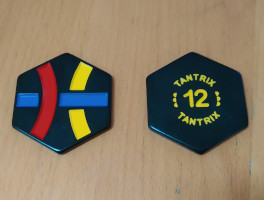
Doing some digging around a while ago I discovered an old puzzle I had as a kid. Tantrix is a set of 56 hexagonal tiles, each with three coloured lines connecting pairs of edges. With these tiles you can solve single-player puzzles, and play games with two or more players.

Discovery Puzzle
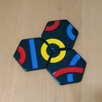
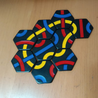
One of the single-player puzzles is the discovery puzzle. With a subset of tiles, the aim is to make a complete loop in a single colour with the constraints that all tiles should be used, and all other touching edges should also match colour.
Each tile is numbered and has a colour on its reverse side – these are used to determine the colour of the loop and which tiles should be used in order to solve a loop of a given size. For example, a loop of size 5 would use all tiles {1, 2, 3, 4, 5}, and the colour should be red (as tile 5 is a red tile).
The player should start with 3 tiles, and increase the loop size each time by introducing a new tile each time – with larger loops being more challenging to solve. The puzzle is solvable up to a loop size of 30.

It’s an interesting puzzle to solve manually. There are also some intricacies that make it interesting to design an algorithm to solve by computer. How might we go about building a solver to complete this puzzle..? 🤔
Generating Solutions
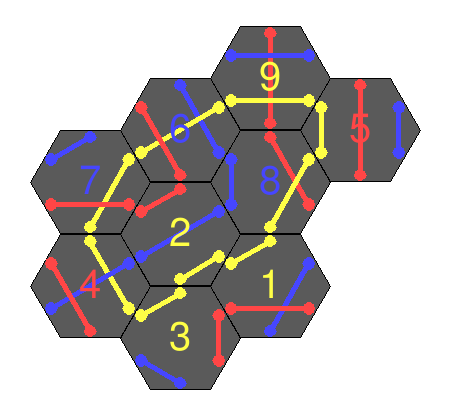
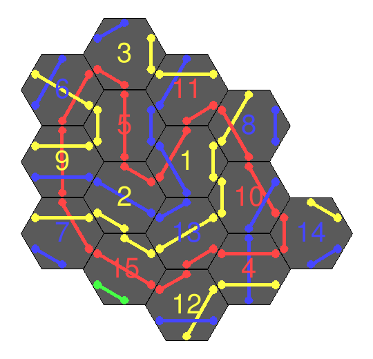
Spoiler – here’s the solved output for some different loop sizes corresponding to the real-life solutions above:
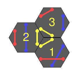
And a visualisation of the intermediate steps of the solver:
Building The Solver
See also the code on GitHub
Algorithm
We’ll approach the problem initially through recursive search with backtracking. Essentially, we will brute force the problem: build a walk piece by piece by attempting every combination of piece next to each other. In a sort of pseudocode:
PROCEDURE solve(remaining_tiles) IS
    IF remaining_tiles = ∅¹ THEN
        RETURN TRUE

    FOR EACH tile IN remaining_tiles DO
        FOR orientation IN {1, 2}² DO
            rotate and place tile to join with current loop end
            IF placement IS valid THEN
                IF solve(remaining_tiles \ {tile}) THEN
                    RETURN TRUE

            unplace tile
        LOOP
    LOOP

    RETURN FALSE
¹ empty set. ² each tile has two endpoints. If the piece is a straight line, we still also need to try both ends, as some of the colours on the edge might end up clashing with other tiles.
Theoretical Analysis
It’s a pretty naive approach to solving the problem. After having placed n tiles we have n-1 tiles which we need to try to connect to continue the walk. For each tile, we have two orientations we need to try. The complexity of building all walks is 2n * n!. However this doesn’t take into account invalid placements such as self-intersections, and non-matching colours that will prune the search greatly. Additionally, only a small subset of these walks will be loops.
In any case, this should be ok for smaller loops, but we might need to be a bit smarter for larger numbers of tiles (tilt head sideways for graph):
n       2^n * n!
3       48
4       384
5       3840
10      3715891200
15      42849873690624000
30      284813089515958324736640819941867520000000
Tiles & Hexagonal Coordinate System
It would be useful to reference the position of tiles within some sort of coordinate system. However the hexagonal shape of the tiles make things a little tricky. In a vertical column, the pieces all have the same horizontal component. But unlike in a cartesian grid, a row isn’t be easily defined.¹
To solve this, we will use a relative coordinate system whereby:
- columns are in ascending x
- even x has only even y
- odd x has only odd y
- (0, 0) is in the top left corner, x and y increase right and down respectively²
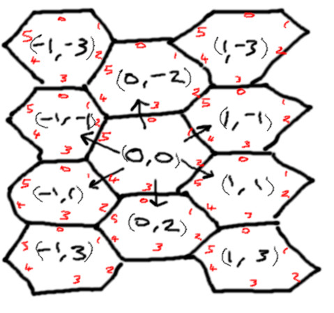
This creates some ‘gaps’ in the coordinate system, but all valid coordinates are correct relative to each other. From any coordinate, it is easy to generate the set of neighbouring coordinates. The tile edges are enumerated clockwise from the ‘top’ edge. The edge of the neighbour tile that touches the current edge has index (edge + 3) MOD 6.
¹How would this change if the corner of a tile was considered “up” instead of the tile edge?
²This is a bit of an arbitrary/counter-intuitive choice, but an ‘increasing y-downwards’ system matches the coordinate system of the images I will need to visualise also later.
Implementation Detail
The solve is written in Python, with Pillow as a dependency to generate the images. The implementation is written in an OOP style across 4 classes
- Tile has some useful methods for manipulating (e.g. rotating and aligning) tiles.
- HexagonBoard keeps track of the current placement state of the tiles. A sparse matrix (DOK) is used to keep track of the tiles. A Python dictionary is keyed by a tuple of tile (x, y) coordinate. This also makes it easier to expand the board in any direction (compared to a matrix by row & column indices) as the search grows.
- RingSolver the implementation of the algorithm itself, with the
solvemethod returning aHexagonBoardof the layout on successful completion - HexagonBoardVisualiser generates some (crude) images of the layout of the board.
We create the tileset at runtime using a CSV datafile, from the data on the tile list on the Tantrix Wikipedia page
Evaluation
The solver in its unoptimised state works well for creating loops with smaller numbers of tiles (19 tiles or fewer). Any more than this, and it starts to take quite a while to find a solution. The graph (note logarithmic scale) below shows the solve time on a standard desktop PC with fitted exponential trend line (R2 = 0.93).
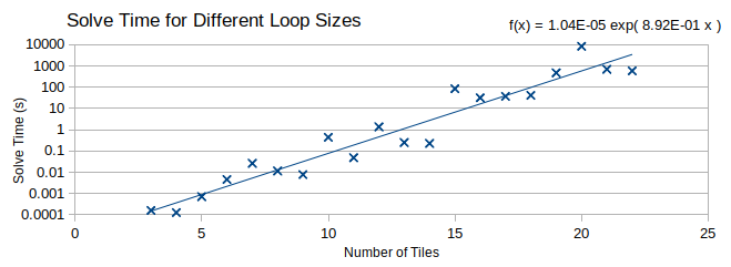
Following this trend, a 30-tile loop would take just over 50 days to solve! It is interesting to note that some larger loops are much quicker to find a solution than the loop one size smaller (e.g. for n=15 and n=16, 84 and 32 seconds respectively). I believe part of this down to the ‘luck’ of tile ordering. In our implementation, note that we always place tile 1 first, and sequentially go through the tiles remaining at each step. If we look at the solutions that were found for n=15, n=16:
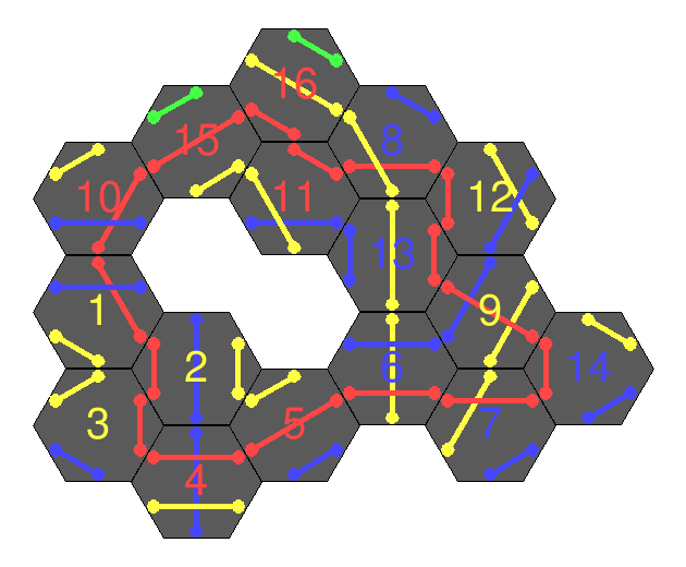
the loop begins (we always place tile 1 first in our implementation) 1-5-3 in the n=15 loop, and 1-2-3-4-5-6-7(!) in the n=16 loop. For n=16 we didn’t need to search for any solutions beginning 1-3, 1-4, 1-5, potentially culling a large portion of the search near the root.
Additionally, note that we return as soon we find the first valid solution. However, multiple solutions may be possible. In the n=16 loop above, we could swap tiles 10 and 4 with still a complete loop and all colours matching. It could be the case too that for a given n, there will be more solutions than for another n. This will likely be partly dependent on the geometry of the tiles available. For an n that allow a less ‘dense’ solution (such as n=16 with its internal hole), there is a greater probability of being able to swap tiles around. This is because there will be more tiles with only two edges touching – fewer edges to clash on a swap. Subsequently, this could lead to more solutions.
Next Steps
Coming soon: in part 2 we will start optimising the algorithm to make the search more efficient so that we can solve larger loops.
